Point Selection in wavelet signal

library(aforoR)
library(ggplot2)
library(tidyr)
library(dplyr)
#> 
#> Attaching package: 'dplyr'
#> The following objects are masked from 'package:stats':
#> 
#>     filter, lag
#> The following objects are masked from 'package:base':
#> 
#>     intersect, setdiff, setequal, union

About this tutorial

In shape analysis, we often end up with high-dimensional functional data, such as wavelet coefficients or radial distances. Identifying which points on these curves are most discriminative for classification is a common challenge. This tutorial illustrates how to use the Hall & Bathia (2012) algorithm to sequentially select the best points to maximize classification accuracy.

1. Scientific Rationale

Functional data analysis (FDA) is essential for capturing the complex geometric information in biological structures like otoliths. However, not all points on a contour or all scales of a wavelet transform carry equal signal for species discrimination. Some points may represent noise or intra-specific variation rather than the inter-specific differences we want to capture.

The selection of a subset of discriminative points is biologically meaningful as it can pinpoint specific anatomical features (e.g., the position of the excisura or the degree of crenulation on the dorsal margin) that define the phenotype (Tuset et al., 2003).

The aforoR package includes an implementation of the component-wise classification algorithm, which avoids the “curse of dimensionality” by selecting points that contribute the most to the separation of groups while minimizing redundancy.

2. Dataset: Aphanopus Wavelets

We will use the included Aphanopus_W5 dataset, which contains wavelet coefficients (scale 5) for two species: Aphanopus carbo and A. intermedius.

data("Aphanopus_W5")
# Target species
species <- Aphanopus_W5$Species

# Prepare data for ggplot2
wavelet_long <- Aphanopus_W5 %>%
    select(Species, starts_with("W")) %>%
    mutate(id = row_number()) %>%
    pivot_longer(cols = starts_with("W"), names_to = "Index", values_to = "Value") %>%
    mutate(Index = as.numeric(gsub("W", "", Index)))

# Professional visualization theme
aforo_theme <- function() {
    theme_minimal() +
        theme(
            legend.title = element_blank(),
            legend.text = element_text(size = 8),
            plot.title = element_text(size = 12, face = "bold", hjust = 0.5),
            axis.title = element_text(size = 10),
            axis.text = element_text(size = 8, color = "black"),
            panel.grid.minor = element_blank(),
            panel.grid.major = element_blank(),
            axis.line = element_line(color = "black", linewidth = 0.3),
            axis.ticks = element_line(color = "black", linewidth = 0.3),
            axis.ticks.length = unit(0.15, "cm")
        )
}

# Visualize the first 10 individuals
ggplot(wavelet_long %>% filter(id <= 10), aes(x = Index, y = Value, group = id, color = Species)) +
    geom_line(linewidth = 0.5) +
    scale_color_manual(values = c("blue", "coral2")) +
    labs(title = "Wavelet Coefficients (Scale 5)", x = "Point Index", y = "Coefficient Value") +
    aforo_theme()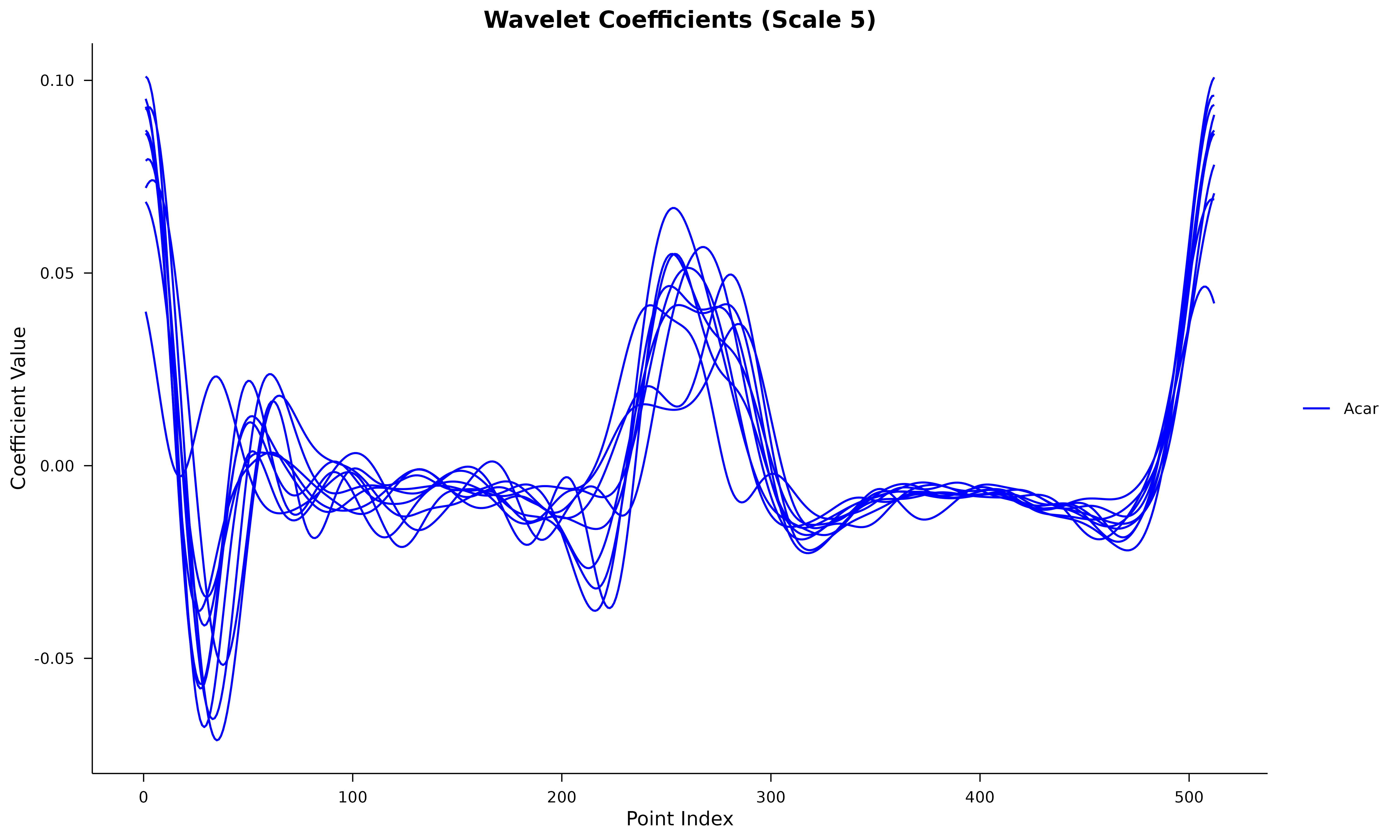

3. Sequential Point Selection

The select_points_hall() function performs a sequential search. It starts by finding the single best point, then the next best in combination with the first, and so on.

Methodology

The algorithm optimizes a classification criterion (e.g., LDA error). It is particularly useful for identifying local features that distinguish phenotypes (Hall & Bathia, 2012).

# Extract wavelet coefficients (columns 3 to 514)
wavelet_data <- Aphanopus_W5[, 3:514]

# Perform selection (finding top 5 points)
result <- select_points_hall(wavelet_data, species,
    method = "lda",
    p = 0.05,
    parallel = FALSE
)

# Professional reporting
cat("Selected indices:", paste(result$selected_indices, collapse = ", "), "\n")
#> Selected indices: 253, 497
cat("Minimum Leave-One-Out Cross-Validation error:", round(result$error_path, 4), "\n")
#> Minimum Leave-One-Out Cross-Validation error: 0.3079 0.2867

4. Final Visualization

Mapping the selected points back to the functional data allows us to identify the specific regions of the otolith that differ between species.

ggplot(wavelet_long, aes(x = Index, y = Value, group = id, color = Species)) +
    geom_line(alpha = 0.1, linewidth = 0.2) +
    geom_vline(xintercept = result$selected_indices, linetype = "dashed", color = "black", alpha = 0.5) +
    geom_point(
        data = wavelet_long %>% filter(Index %in% result$selected_indices),
        aes(x = Index, y = Value), alpha = 0.5, size = 1
    ) +
    scale_color_manual(values = c("blue", "coral2")) +
    labs(
        title = "Discriminative Point Localization",
        subtitle = paste("Indices selected:", paste(sort(result$selected_indices), collapse = ", ")),
        x = "Index", y = "Value"
    ) +
    aforo_theme()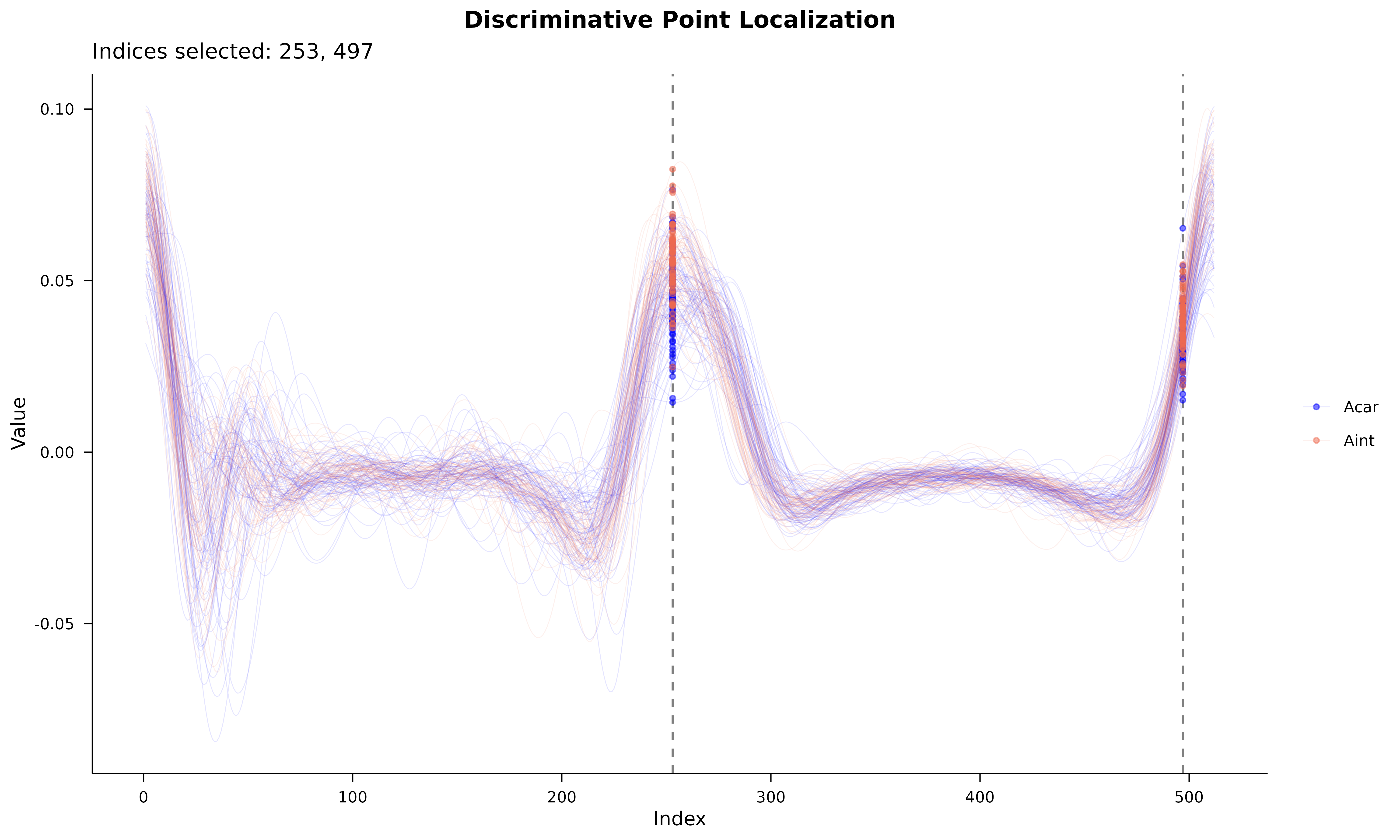

References

Hall, P., & Bathia, N. (2012). Componentwise classification and clustering of functional data. Biometrika, 99(2), 297-313.
Parisi-Baradad, V., et al. (2005). Otolith shape contour analysis using mathematical descriptors. Computers in Biology and Medicine.
Tuset, V. M., et al. (2003). Morphometric similarity of the otoliths of any species of the Serranus. Journal of Fish Biology.

Jose Luis Otero Ferrer