Lobe Analysis with Wavelets
Víctor Manuel Tuset
2025-11-27
Source:vignettes/Analyzing_Lobes.Rmd
Analyzing_Lobes.RmdAbout this tutorial
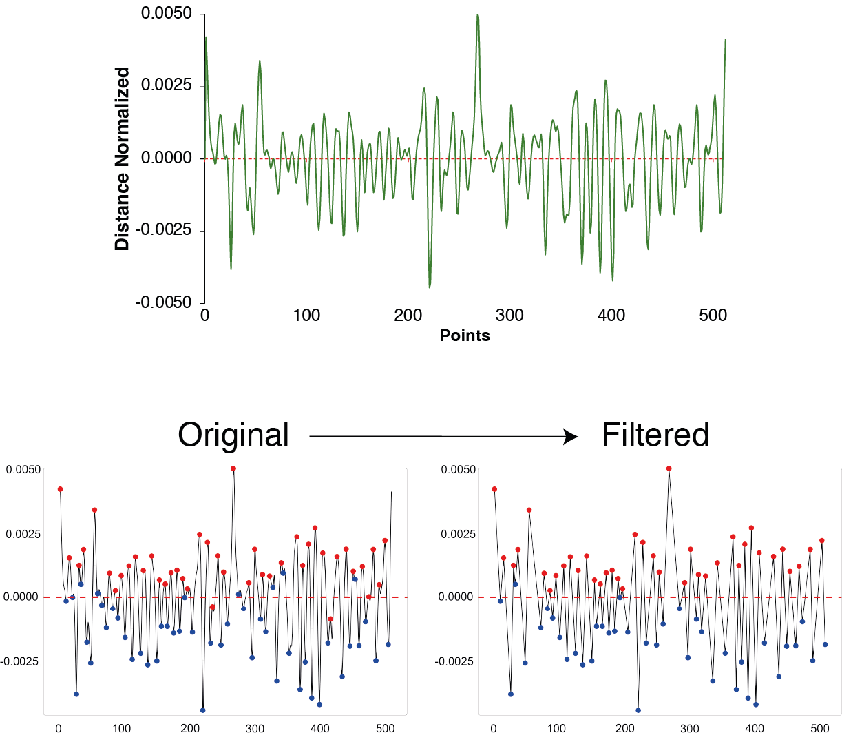
This tutorial shows how to quantify the number, depth, height, and crenulation of lobes from the 2nd scale of wavelet function. This approach is specially useful when wavelets (>3rd scale) and Fourier descriptors excessively smooth the contour.
Framework
Definitions:
- The lobe depth (LD) is estimated as: LDi=1…n = normalized distance (Peaki - Valleyi), where LD1 = Peak1 - Valley1, LD2 = Peak2 - Valley2, and so on,
- The height lobes (HD) is estimated as: HDi=1…n = normalized distance (Peaki - Valleyi), where HD1 = Peak1 - Peak2, HD2 = Peak2 - Peak3, and so on,
- The crenulation lobes (LC) is estimated as: LDi=1…n = distance between points (Peakip - Peakip), where LD1 = Peak1p - Peak2p, LD2 = Peak2p - Peak3p, and so on.
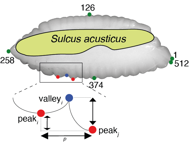
Premises:
- After a peak must have a valley, the first point of the wavelets is always the first peak,
- The second peak (or valley) of two consecutive peaks (or valley) is always removed,
- The last value is always a valley.
To estimate the 2nd scale of wavelet function and modify it following premises.
Estimating lobes
library(aforoR)
library(dplyr)
library(pracma)

# Use built-in Aphanopus_W5 dataset
data(Aphanopus_W5)

# Prepare Data: Columns should be individuals, rows should be indices
# We take first 5 individuals as an example
examples <- Aphanopus_W5[1:5, ]
Data_coeffs <- t(examples[, 3:514]) # Transpose coefficients
Data <- cbind(1:512, Data_coeffs) # Add index column
colnames(Data)[1] <- "Index"
# Select peaks and valleys for multiple images

# Step 1
fpeaks <- function(Data) {
  peaks <- findpeaks(Data, nups = 3, ndowns = 1) # user define
  # Get the real distance for the first point
  first_distance <- Data[1] # First data point as the real distance
  # Add the first point as a peak
  peaks <- rbind(c(first_distance, 1), peaks) # First point (time = 1) as a peak with a distance of 0
  peaks <- peaks[!duplicated(peaks[, 2]), ] # Remove consecutive duplicate peaks (same position)
  return(peaks)
}

fvalley <- function(Data) {
  valleys <- findpeaks(-Data, nups = 3, ndowns = 1) # Use negative values to detect valleys
  valleys <- valleys[!duplicated(valleys[, 2]), ] # Remove consecutive duplicate valleys (same position)
  return(valleys)
}
# =======================================================
# Step 2: apply findpeaks to all columns
peaks_listData <- apply(Data[, -1], 2, fpeaks)
valleys_listData <- apply(Data[, -1], 2, fvalley)
# =======================================================
# Step 3: Initialize a list to store the peak-valley distances for each column
peak_valley_distances <- list()

# Loop through each sample
for (i in seq_along(peaks_listData)) {
  # Extract peak data
  peaks <- peaks_listData[[i]]
  valleys <- valleys_listData[[i]]

  # Adjust the distance for valleys (negated in findpeaks)
  valleys[, 1] <- -valleys[, 1]

  # Combine into one data frame
  combined <- data.frame(
    position = c(peaks[, 2], valleys[, 2]),
    distance = c(peaks[, 1], valleys[, 1]),
    type = c(rep("peak", nrow(peaks)), rep("valley", nrow(valleys)))
  )

  # Order by position
  combined_sorted <- combined[order(combined$position), ]
  peak_valley_distances[[i]] <- combined_sorted
}

peak_valley_distances[[1]]
## position distance type
## 1 1 0.092349559 peak
## 10 35 -0.071272178 valley
## 2 65 0.018164486 peak
## 11 125 -0.013183946 valley
## 3 164 -0.006526793 peak
## 12 185 -0.014534450 valley
## 4 207 -0.006215359 peak
## 13 220 -0.008167561 valley
## 5 260 0.051321822 peak
## 14 310 -0.015885427 valley
## 6 342 -0.008276288 peak
## 15 355 -0.009408289 valley
## 7 372 -0.007344856 peak
## 16 383 -0.007844535 valley
## 8 401 -0.005555449 peak
## 17 429 -0.011129436 valley
## 9 436 -0.010976275 peak
## 18 461 -0.015779525 valley
# =======================================================
# Step 4:Function to eliminate consecutive peaks or valleys with the same type
eliminate_consecutive <- function(peak_valley_data) {
  # Initialize the cleaned data with the first row
  cleaned_data <- peak_valley_data[1, , drop = FALSE] # Keep the first row

  for (j in 2:nrow(peak_valley_data)) {
    # Get the current and previous row
    current_row <- peak_valley_data[j, , drop = FALSE]
    prev_row <- cleaned_data[nrow(cleaned_data), , drop = FALSE]

    # Only add the row if the "type" is different from the previous row's "type"
    if (current_row$type != prev_row$type) {
      cleaned_data <- rbind(cleaned_data, current_row) # Add the current row
    } else {
      # If the same type (consecutive peaks or valleys), compare the absolute values of distance
      if (abs(current_row$distance) > abs(prev_row$distance)) {
        # Keep the row with the larger absolute value (discard the previous one)
        cleaned_data <- cleaned_data[-nrow(cleaned_data), , drop = FALSE] # Remove the previous row
        cleaned_data <- rbind(cleaned_data, current_row) # Add the current row
      }
    }
  }

  # Order the cleaned data by position (ascending order)
  cleaned_data_sorted <- cleaned_data[order(cleaned_data$position), ]

  return(cleaned_data_sorted)
}

# Loop through and clean consecutive peaks/valleys
for (i in seq_along(peak_valley_distances)) {
  peak_valley_data <- peak_valley_distances[[i]]
  peak_valley_distances[[i]] <- eliminate_consecutive(peak_valley_data)
}

peak_valley_distances[[1]]
## position distance type
## 1 1 0.092349559 peak
## 10 35 -0.071272178 valley
## 2 65 0.018164486 peak
## 11 125 -0.013183946 valley
## 3 164 -0.006526793 peak
## 12 185 -0.014534450 valley
## 4 207 -0.006215359 peak
## 13 220 -0.008167561 valley
## 5 260 0.051321822 peak
## 14 310 -0.015885427 valley
## 6 342 -0.008276288 peak
## 15 355 -0.009408289 valley
## 7 372 -0.007344856 peak
## 16 383 -0.007844535 valley
## 8 401 -0.005555449 peak
## 17 429 -0.011129436 valley
## 9 436 -0.010976275 peak
## 18 461 -0.015779525 valley
# =======================================================
# Step 5: Function to remove the last row if it is a peak
remove_last_peak <- function(peak_valley_data) {
  # Check if the last row is a "peak"
  if (nrow(peak_valley_data) > 0 && peak_valley_data[nrow(peak_valley_data), "type"] == "peak") {
    peak_valley_data <- peak_valley_data[-nrow(peak_valley_data), ]
  }

  return(peak_valley_data)
}

# Loop through each sample and remove the last peak if it exists
for (i in seq_along(peak_valley_distances)) {
  peak_valley_data <- peak_valley_distances[[i]]

  # Eliminate consecutive peaks or valleys
  peak_valley_data <- eliminate_consecutive(peak_valley_data)

  # Remove the last peak
  peak_valley_distances[[i]] <- remove_last_peak(peak_valley_data)
}

# Preview cleaned data
peak_valley_distances[[1]]
## position distance type
## 1 1 0.092349559 peak
## 10 35 -0.071272178 valley
## 2 65 0.018164486 peak
## 11 125 -0.013183946 valley
## 3 164 -0.006526793 peak
## 12 185 -0.014534450 valley
## 4 207 -0.006215359 peak
## 13 220 -0.008167561 valley
## 5 260 0.051321822 peak
## 14 310 -0.015885427 valley
## 6 342 -0.008276288 peak
## 15 355 -0.009408289 valley
## 7 372 -0.007344856 peak
## 16 383 -0.007844535 valley
## 8 401 -0.005555449 peak
## 17 429 -0.011129436 valley
## 9 436 -0.010976275 peak
## 18 461 -0.015779525 valley
# =======================================================
# Step 6: Estimating measurements: HD and LC
# Initialize a list to store the results
HDLC_df <- list()

# Loop through each element of peak_valley_distances
for (i in seq_along(peak_valley_distances)) {
  # Extract the current case
  HDLC <- peak_valley_distances[[i]]

  # Filter only peaks
  peaks_only <- HDLC[HDLC$type == "peak", ]

  if (nrow(peaks_only) > 1) {
    # Compute the height difference between consecutive peaks
    peak_diff_HD <- peaks_only$distance[-nrow(peaks_only)] - peaks_only$distance[-1]

    # Compute the (absolute) position difference between consecutive peaks
    peak_diff_LC <- abs(peaks_only$position[-nrow(peaks_only)] - peaks_only$position[-1])

    # Create a data frame for this case
    df_case <- data.frame(
      Peak_from = peaks_only$position[-nrow(peaks_only)],
      Peak_to = peaks_only$position[-1],
      HD = peak_diff_HD,
      LC = peak_diff_LC
    )
  } else {
    df_case <- data.frame(Peak_from = NA, Peak_to = NA, HD = NA, LC = NA)
  }

  # Store the result in the list
  HDLC_df[[i]] <- df_case
}

# Access the first case
HDLC_df[[1]]
## Peak_from Peak_to HD LC
## 1 1 65 0.0741850731 64
## 2 65 164 0.0246912788 99
## 3 164 207 -0.0003114337 43
## 4 207 260 -0.0575371814 53
## 5 260 342 0.0595981109 82
## 6 342 372 -0.0009314322 30
## 7 372 401 -0.0017894072 29
## 8 401 436 0.0054208259 35
# =======================================================
# Step 7: Estimating values: LD
# Initialize a list to store the results
LD_df <- list()

# Loop through each element of peak_valley_distances
for (i in seq_along(peak_valley_distances)) {
  # Extract the current case (data frame with position, distance, type)
  LD_data <- peak_valley_distances[[i]]

  # Extract peaks and valleys separately
  peaks <- LD_data[LD_data$type == "peak", ]
  valleys <- LD_data[LD_data$type == "valley", ]

  # Ensure the same number of peaks and valleys for pairing:
  # LD_i = Peak_i - Valley_i
  n_pairs <- min(nrow(peaks), nrow(valleys))

  if (n_pairs > 0) {
    LD_values <- peaks$distance[1:n_pairs] - valleys$distance[1:n_pairs]

    df_case <- data.frame(
      Peak_position = peaks$position[1:n_pairs],
      Valley_position = valleys$position[1:n_pairs],
      LD = LD_values
    )
  } else {
    df_case <- data.frame(Peak_position = NA, Valley_position = NA, LD = NA)
  }

  # Store the result for this case
  LD_df[[i]] <- df_case
}

# Access the first case
LD_df[[1]]
## Peak_position Valley_position LD
## 1 1 35 0.163621737
## 2 65 125 0.031348432
## 3 164 185 0.008007658
## 4 207 220 0.001952202
## 5 260 310 0.067207250
## 6 342 355 0.001132000
## 7 372 383 0.000499679
## 8 401 429 0.005573987
## 9 436 461 0.004803250From HDLC_df and LD_df, users can perform
their analyses.